The Limits of AI Image Colorization: A Companion

I wrote a short article for hyperallergic.com. As it’s a website for a general audience, it’s a quite short article without technical details. As a companion here, I wanted to write out some more of the details about deep learning algorithms for image colorization.

This post is a little bit rushed, as the article is coming out soon, but I thought it would be helpful to provide more information for those who are interested. All of my information about the particular colorization model DeOldify is based on the github, I’m not a colorization researcher myself (though I have worked with conditional GANs and pix-to-pix models before, and know some things about color and history), so take what I say with a grain of salt.

I’m going to try to write concisely in technical detail, which unfortunately means this isn’t going to be a good explanation for people who haven’t encountered machine learning before. You’re still free to follow along, but some of the words and ideas might not make sense without like, a semester course of context.

Image Colorization

The image colorization problem, like many other machine learning problems in computer vision, is generally framed as an “inverse problem” of recovering high dimensional data (a color image) from its low-dimensional representation (a grayscale image). It’s also a pixel-to-pixel problem: we want to predict a label (color) for each pixel.

These two qualities make it quite similar to two highly studied vision problems: semantic segmentation and depth estimation. Semantic segmentation asks for an algorithm to segment an image: group the pixels based on the objects to which they belong, and then label each segment with a semantic category, indicating which kind of object they depict. Depth estimation asks for an algorithm to reason about the 3D nature of a scene and, for each pixel, identify how far away the object producing that pixel was from the camera.

These problems are all ill-posed. Unlike other ill-posed problems like linear regression which are over-constrained (they are kind of like systems of equations with more equations than unknowns), colorization, semantic segmentation and depth estimation are under-constrained (we have a relatively small number of equations, one per pixel, and too many unknowns, three per pixel). We can’t shortcut the problem by combining all of our pixels together, either, as multiple pixels in the same image with the same grayscale value might map to different colors. This means we need to turn to machine learning and use training images.

Existing work for these sorts of pixel-to-pixel problems was originally done with a class of statistical models called Markov random fields, but since the “U-Net” deep neural network architecture was proposed by Ronnenberger et al. in 2015, deep neural networks have been the state of the art.

U-Net for Colorization

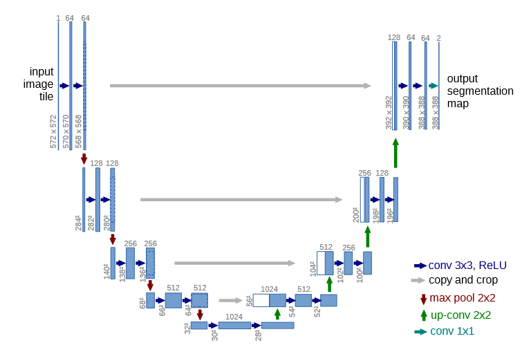
There are plenty of posts online explaining how these models work, so I won’t try to explain the details. The gist is that while ordinary convolutional neural networks use convolution and pooling operations to progressively reduce the width and height of an image while increasing the number of convolutional filters until reaching a classifier, U-net architectures then do the same thing again, in reverse. They take a representation with small width and height and use transposed convolutions to return to an image-shaped representation. These models are trained with either a classification or regression loss, similarly to a more conventional CNN, except the loss function is applied on each pixel individually.

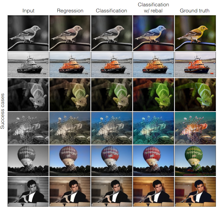
You would think that colorization would work similarly to either depth estimation or semantic segmentation, but it turns out classification and regression losses don’t produce very good looking colorizations. As the figure below from Richard Zhang, Philip Isola and Alexi Efros’ fantastic 2016 paper “Colorful Image Colorization” shows, classification and regression losses lead to bland colorizations.

Conditional GANs

Instead of using regression and classification losses, however, there is a better approach which Philip Isola introduced to pixel-to-pixel problems the next year: conditional generative adversarial networks. These models look exactly the same as U-Net in terms of their model architecture, but instead of a simple hand-designed loss function, they use another convolutional neural network to approximate the loss function.

This idea comes from Ian Goodfellow’s Generative Adversarial Networks (GANs). The gist is that there are two neural networks. One network (the “generator”) learns to generate new data from scratch and the other one (the “discriminator”) learns to tell the difference between real data and data generated by the generator. They are trained competitively: the generator is then trained to fool the discriminator, and they are both iteratively retrained. Eventually, if everything goes according to plan, the generator will only generate things which are indistinguishable from the training data.

Conditional generative adversarial networks are the same thing, except the generator isn’t generating data from scratch. Instead, it generates data conditioned on some input. In our case, the input to the generator is a black and white image while the output is a color image. The discriminator then has to distinguish between real color images and colorized ones.

While GANs sound great in theory, they often just don’t work. Usually either the discriminator gets too good too fast and the generator can’t learn anything, or the generator only learns how to make one image (“mode collapse”). To prevent this problem, researchers have proposed a variety of other GAN models which are more reliable, especially for conditional GAN problems.

Perceptual Loss

One trick that GAN researchers use is additional loss functions besides the adversarial loss coming from the discriminator. A particularly clever option, which they use here, is called the “perceptual” loss. Whose perception, you might ask? Well, another neural network.

The idea here is that we can repurpose an existing model (usually a CNN classifier trained on the ImageNet dataset) as a feature extractor, and treat the hidden activations of the last layer as a vector space, then measure euclidean distance in that space between the generated image and the target image as an additional loss function. Because this is a loss in classifier “feature-space” it’s also called “feature loss.” That loss is zero only if the two images are identical, in the “eyes” of the pretrained model.

This method tends to measure something similar to losses like pixel-wise error, but for whatever reason works better when training conditional GANs. The two losses are usually in opposition, as the GAN wants to generate as realistic of an image as possible, while the perceptual loss ties it back to the training input/output pair. Getting back to colorization, the adversarial loss encourages the colorization to have unusual colors which are bold enough to trick the discriminator, while the perceptual loss encourages it to have muted colors which are more likely given the training data.

Side note: this pattern, of using loss functions with two components, connects to a deeply important theoretical concept in machine learning. Machine learning models (like all statistical models) have a natural tradeoff between two properties, bias (which is not the same as algorithm bias in the real-world sense) and variance. High bias models resist training and tend to underfit while high variance models train too easily and tend to overfit. There is a “sweet spot” in the middle where the model actually learns to solve the problem. Many, many machine learning models use a combination of capacity (which increases variance) and regularization (which increases bias) to control this tradeoff. With conditional GANs, the perceptual loss is a regularizing force, which encourages safe choices, while the adversarial loss encourages a better fit to the data.

Jason Antic’s DeOldify Model

The model which is being used online is Jason Antic’s DeOldify. This model is unusual, in that it uses the amount of time spent training the GAN as a tradeoff between the adversarial and perceptual losses, rather than some tradeoff hyperparameter.

The backbone model is a variant on the U-Net GAN which makes use of self-attention, an alternative to convolutional layers which improves long-distance coherence. For more information check out the SAGAN paper. Antic trains three versions of this model, primarily only using a perceptual loss (which he calls feature loss), but with a little bit of adversarial training at the end to make the images less bland. One version gets 5 iterations of generator-discriminator training, the second version gets 3 and the third version only gets 1.

That means the first model produces colorful “artistic” images, but often gets the colors of common things like plants, buildings and the sky clearly wrong. The second model is “stable” since it will make fewer bold color choices. The third model is best for “video” since it is highly consistent from image to image.

An Example

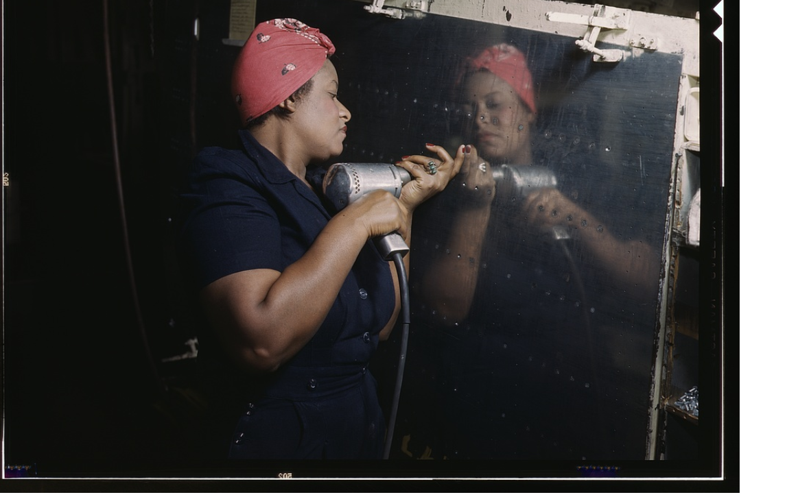
To explore how this model works in practice, let’s use an example. First, consider this photograph. It was taken in color in 1943 by the photography Alfred T. Palmer while working for the US Government, and is preserved in the Library of Congress:

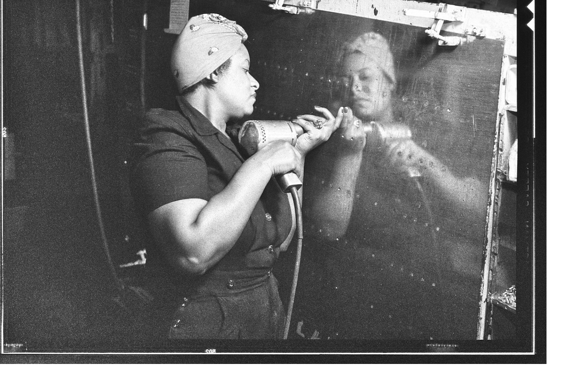
I used an image editor to convert that photo to grayscale:

And then used the “stable” version of DeOldify to colorize it:

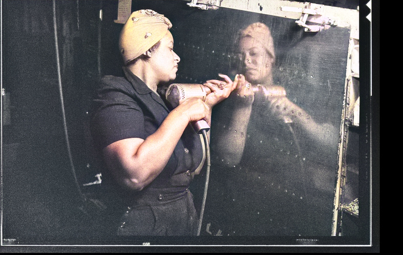
There’s clearly a problem here. The woman’s skin is lightened, her bandana is yellow instead of red and her dress is gray instead of navy blue. Interestingly, the model was able to colorize her reflection similarly, though the bandana is a slightly different shade of yellow. This is a single example of a very general bias which deep learning-based colorization models have towards bland colors.

Why So Bland?

So all of the modeling decisions I described above seem very reasonable, so why do we observe a bias towards bland colors when colorizing historical photos? Well, there are lots of reasons. Let’s go through some.

First, this sort of model needs to be trained on a large image dataset. For practical reasons, ML researchers tend to use ImageNet. ImageNet has a variety of well-known biases, especially with respect to people, that its developers are trying to remedy. It also only contains modern photos which were collected from Flickr in the late 2000’s. Further, it’s not a very representative dataset of photographs in general, as it is built to be a classification set with only one promenant object per photo.

Second, the model just doesn’t have any sort of historical or cultural knowledge to rely on when making color decisions. Different historical films have different color sensitivities, and age differently. Applying a grayscale conversion to a modern digital photo is easy and fast, but it doesn’t provide any training data to help the model recognize those hints. Further, we have historical records and artifacts which in conjunction with the place and time the photo was taken, might give us more information about the colors of human-made contents of a photo, like clothes.

Third, the model doesn’t have a good sense of color theory. Certain colors “go well” together, and predicting exactly when colors do and don’t is a very difficult statistical problem. Check out my previous posts on this topic if you’re interested. The only sense of color theory which is embedded in this model would have had to be learned by the classifier used for perceptual loss, but the difference between good color schemes and bad ones just isn’t relevant to ImageNet classification.

All of these explanations give reasons why the model might have learned a more limited model of the world, which might make it default to a bland colorization strategy in the case of unfamiliar data, but it doesn’t quite get at the concept of bias, in the social sense.

Algorithm Bias

Algorithms are biased in the real-world sense when they perform differently in different situations in such a way which reinforces existing soical inequality. Typical examples of algorithm bias include racial stereotypes in search engine recommendations, hiring algorithms which learn to reject the resumes of women or medical software which underestimates the sickness of black patients. What does a preference towards bland colors in image colorization have to do with algorithm bias?

Well, for one, it means that these colorization algorithms, if used uncritically, will lighten the skin of dark-skinned people, effectively denying them representation in the colorized photographic record. Bland colorization also takes the vibrant clothes, architecture and food of historical peoples, propagating the myth that bright colors are a modern invention. Such a practice is cultural erasure which reinterprets the past, injecting new information and changing our concept of history.

This is an example of emergent bias, a term which originates in the work of Friedman and Nissenbaum. Instead of the bias coming from a clearly incorrect decision, it just emerges out of a combination of reasonable technical decisions and real-world context. But that doesn’t mean it’s not a problem. There is a serious imperative for researchers in the image colorization space to think about these issues and find alternatives which produce reasonable colorizations without dulling the past. I’m not quite sure what that would be, but it’s not unreasonable to imagine, for example, an interactive GAN colorization tool which asks the user questions like, “which of these colors would be more reasonable for this woman’s skin?” instead of just choosing an estimate.

In general, though, we need to seriously reconsider our trust in digital photographs without clear provenance. There’s no way to make colorization algorithms like this one just stop existing, and no way to know whether a given grid of pixels on the Internet is a genuine historical photo or a fictional result from a colorization algorithm. Technologies like DeepFakes allow highly sophisticated synthetic and doctored images, and the general success of online GAN-based face generators means that photorealism isn’t enough to treat photos as evidence.

Thanks for reading!

Hopefully this explanation was helpful. I’m happy to answer questions at the email address in the sidebar, as well as make corrections if I’ve gotten any technical details wrong here. I’ve also been hard at work in grad school and have a couple different projects which are going to make a blog appearance if I ever get around to writing them. Stay tuned!